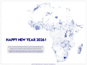
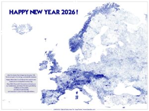
Like the rivers that shape landscapes, fish farms are part of a living, sustainable balance.
Happy New Year from the KAMAHU Team to all those who watch over aquaculture ecosystems every day.
May 2026 flow with the same continuity as our waterways, and may this new year bring stability to the ponds, serenity in monitoring, and success in your farming operations.
Here is the code we used to draw the map of waterways for America. It’s the same logic for Europe, Africa and Asia.
NB : We work on Linux. You’ll find below the command lines.

1) Download the last version from OSM for the continent :
wget -O north-america-latest.osm.pbf https://download.geofabrik.de/north-america-latest.osm.pbf
wget -O north-america-latest.osm.pbf.md5 https://download.geofabrik.de/north-america-latest.osm.pbf.md5
md5sum -c north-america-latest.osm.pbf.md5
wget -O south-america-latest.osm.pbf https://download.geofabrik.de/south-america-latest.osm.pbf
wget -O south-america-latest.osm.pbf.md5 https://download.geofabrik.de/south-america-latest.osm.pbf.md5
md5sum -c south-america-latest.osm.pbf.md5
NB : Files can be large, so we use –continue –no-cache in case of micro-interruptions.
Check integrity of the file :
md5sum -c africa-latest.osm.pbf.md5
You should get
africa-latest.osm.pbf: OK
If this not the case, just remove both files and re-download.
NB : Sometimes, you need to rename the .osm.pbf file to match the .md5 file.
2) Filter waterways :
cat > waterway-filter.txt << ‘EOF’
w/waterway=river
w/waterway=stream
w/waterway=canal
#w/waterway=drain
#w/waterway=ditch
EOF
NB : We comment drains and ditches; otherwise would the file much too big.
osmium tags-filter north-america-latest.osm.pbf -e waterway-filter.txt -o waterways_north_america.osm.pbf --overwrite
osmium tags-filter south-america-latest.osm.pbf -e waterway-filter.txt -o waterways_south_america.osm.pbf --overwrite
3) Export GeoJSONSeq
osmium export waterways_north_america.osm.pbf -f geojsonseq -o waterways_north_america.geojsons --overwrite
osmium export waterways_south_america.osm.pbf -f geojsonseq -o waterways_south_america.geojsons --overwrite
4) Concatenate (stream)
cat waterways_north_america.geojsons waterways_south_america.geojsons > waterways_america.geojsons
5) Render points Datashader (low RAM)
Since we built this map on a small PC, we had to minimize the size of the files and the resources that had to be mobilized.
Create a file render_america_points.py with
cat > render_america_points.py << 'EOF'
import json
import numpy as np
import pandas as pd
import datashader as ds
import datashader.transfer_functions as tf
from datashader.utils import lnglat_to_meters
INP = “waterways_america.geojsons”
OUT = “waterways_america.png”
minlon, minlat, maxlon, maxlat = -170.0, -60.0, -25.0, 83.0
x0, y0 = lnglat_to_meters(minlon, minlat)
x1, y1 = lnglat_to_meters(maxlon, maxlat)
W, H = 7000, 7000
cvs = ds.Canvas(plot_width=W, plot_height=H, x_range=(x0, x1), y_range=(y0, y1))
CHUNK_PTS = 3_000_000
xs = np.empty(CHUNK_PTS, dtype=”float64″)
ys = np.empty(CHUNK_PTS, dtype=”float64″)
n = 0
agg = None
STRIDE = 1
def flush():
global n, agg
if n == 0:
return
df = pd.DataFrame({“x”: xs[:n], “y”: ys[:n]})
a = cvs.points(df, “x”, “y”, agg=ds.count())
agg = a if agg is None else (agg + a)
n = 0
def add_coords(coords):
global n
if not coords:
return
for i in range(0, len(coords), STRIDE):
pt = coords[i]
if not pt or len(pt) < 2:
continue
X, Y = lnglat_to_meters(pt[0], pt[1])
xs[n] = X
ys[n] = Y
n += 1
if n >= CHUNK_PTS:
flush()
with open(INP, “r”, encoding=”utf-8″, errors=”ignore”) as f:
for line in f:
line = line.strip()
if not line:
continue
try:
feat = json.loads(line)
except json.JSONDecodeError:
continue
geom = feat.get(“geometry”)
if not geom:
continue
t = geom.get(“type”)
if t == “LineString”:
add_coords(geom.get(“coordinates”))
elif t == “MultiLineString”:
for coords in geom.get(“coordinates”) or []:
add_coords(coords)
flush()
img = tf.shade(agg, how=”eq_hist”)
img.to_pil().save(OUT)
print(“OK ->”, OUT)
EOF
6) Launch
export PYTHONNOUSERSITE=1
source .venv/bin/activate
python render_america_points.py
7) Cleaning
Don’t forget to remove the files in order to free space (several tens of gigabytes)
rm -f north-america-latest.osm.pbf* south-america-latest.osm.pbf*
rm -f waterways_north_america.osm.pbf waterways_south_america.osm.pbf
rm -f waterways_north_america.geojsons waterways_south_america.geojsons
Here is the result with some tiles that seem to be uncompleted :

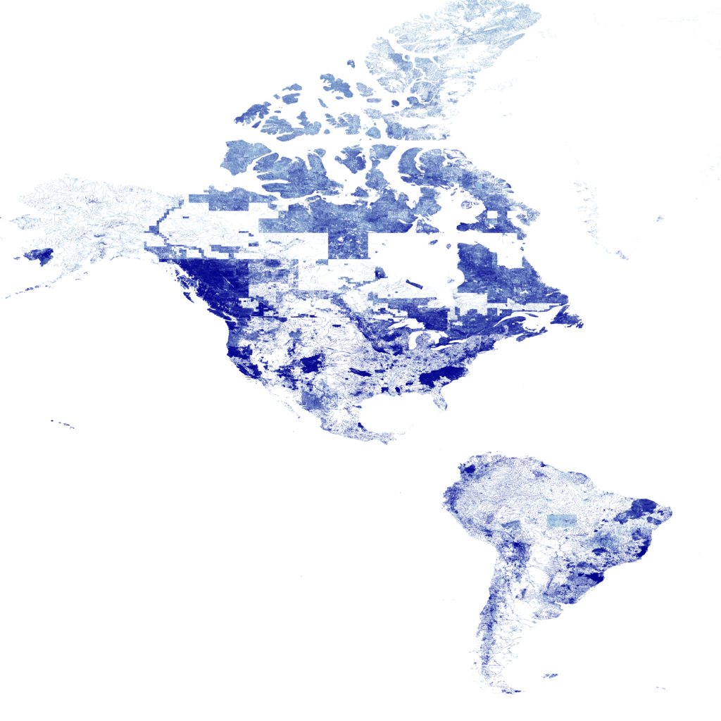
It is interesting to observe that North America appears here as a set of discontinuous “tiles.”
In reality, this stems from the origin of the OSM data, which has heterogeneous coverage.
Some areas (the United States, southern Canada) are extremely well mapped,
while others (northern Canada, Alaska, boreal regions) are very incomplete.
Contributors often import data in blocks (basins, provinces, local projects), which results in dense areas and nearly empty ones, with rectangular or polygonal outlines.
The initial files used, which come from Geofabrik, are themselves aggregated from regional sub-extracts. The discontinuity is therefore already present in the PBF, and the effect is amplified by the Datashader rendering.
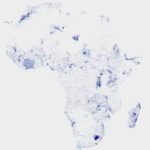
In Europe, OSM coverage is very homogeneous. In Africa, it is patchy but more “organic.” In the Americas, the contrasts are stark and produce this mosaic effect. The resulting map therefore shows the geography of human contribution to OSM. It is more a map of the density of hydrological mapping than a map solely of rivers.
If you’re interested in our skills in map design or python coding, get in touch with us.


